What are GANs?
Deep neural networks are used mainly for supervised learning: classification or regression. Generative Adversarial Networks or GANs, however, use neural networks for a very different purpose: Generative modeling.
Generative Modeling is generating examples that plausibly could have been drawn from the original dataset.
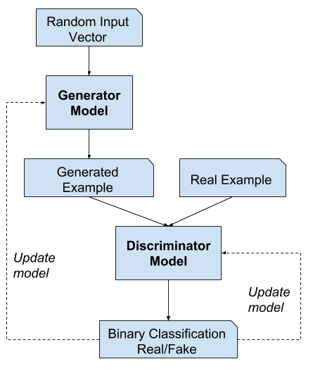
Working of GANs can be explained by the following flowchart:

Dataset
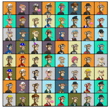
We will be using a dump of all images from the famous Bored Apes Yacht Club (BAYC) NFT.

Making dataset ready for training
Let’s load this dataset using the ImageFolder class from torchvision. We will also resize and crop the images to 64x64 px, and normalize the pixel values with a mean & standard deviation of 0.5 for each channel. This will ensure that pixel values are in the range (-1, 1), which is more convenient for training the discriminator.
import os
from torch.utils.data import DataLoader
from torchvision.datasets import ImageFolder
import torchvision.transforms as T
import torch
from torchvision.utils import make_grid
import matplotlib.pyplot as plt
%matplotlib inline

DATA_DIR = '../input/bored-apes-yacht-club/'
print(os.listdir(DATA_DIR))
image_size = 64
batch_size = 128
stats = (0.5, 0.5, 0.5), (0.5, 0.5, 0.5)
train_ds = ImageFolder(DATA_DIR, transform=T.Compose([
    T.Resize(image_size),
    T.CenterCrop(image_size),
    T.ToTensor(),
    T.Normalize(*stats)]))

train_dl = DataLoader(train_ds, batch_size, shuffle=True, num_workers=2, pin_memory=True)

def denorm(img_tensors):
    return img_tensors * stats[1][0] + stats[0][0]

def show_images(images, nmax=64):
    fig, ax = plt.subplots(figsize=(8, 8))
    ax.set_xticks([]); ax.set_yticks([])
    ax.imshow(make_grid(denorm(images.detach()[:nmax]), nrow=8).permute(1, 2, 0))

def show_batch(dl, nmax=64):
    for images, _ in dl:
        show_images(images, nmax)
        break;
Lets see a sample from dataset -

Discriminator Network
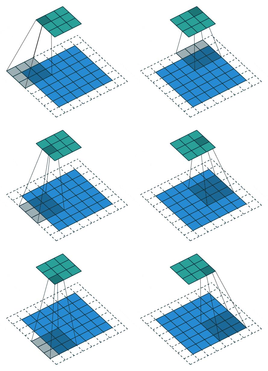
The discriminator takes an image as an input, and tries to classify it as “real” or “generated”. In this sense, it’s like any other neural network. We’ll use a convolutional neural network (CNN) which outputs a single number output for every image. We’ll use a stride of 2 to progressively reduce the size of the output feature map.

import torch.nn as nn

discriminator = nn.Sequential(
    # in: 3 x 64 x 64

    nn.Conv2d(3, 64, kernel_size=4, stride=2, padding=1, bias=False),
    nn.BatchNorm2d(64),
    nn.LeakyReLU(0.2, inplace=True),
    # out: 64 x 32 x 32

    nn.Conv2d(64, 128, kernel_size=4, stride=2, padding=1, bias=False),
    nn.BatchNorm2d(128),
    nn.LeakyReLU(0.2, inplace=True),
    # out: 128 x 16 x 16

    nn.Conv2d(128, 256, kernel_size=4, stride=2, padding=1, bias=False),
    nn.BatchNorm2d(256),
    nn.LeakyReLU(0.2, inplace=True),
    # out: 256 x 8 x 8

    nn.Conv2d(256, 512, kernel_size=4, stride=2, padding=1, bias=False),
    nn.BatchNorm2d(512),
    nn.LeakyReLU(0.2, inplace=True),
    # out: 512 x 4 x 4

    nn.Conv2d(512, 1, kernel_size=4, stride=1, padding=0, bias=False),
    # out: 1 x 1 x 1

    nn.Flatten(),
    nn.Sigmoid())
Generator Network
The input to the generator is typically a vector or a matrix of random numbers (referred to as a latent tensor) which is used as a seed for generating an image. The generator will convert a latent tensor of shape (128, 1, 1) into an image tensor of shape 3 x 28 x 28.
import torch.nn as nn
generator = nn.Sequential(
    # in: latent_size x 1 x 1

    nn.ConvTranspose2d(latent_size, 512, kernel_size=4, stride=1, padding=0, bias=False),
    nn.BatchNorm2d(512),
    nn.ReLU(True),
    # out: 512 x 4 x 4

    nn.ConvTranspose2d(512, 256, kernel_size=4, stride=2, padding=1, bias=False),
    nn.BatchNorm2d(256),
    nn.ReLU(True),
    # out: 256 x 8 x 8

    nn.ConvTranspose2d(256, 128, kernel_size=4, stride=2, padding=1, bias=False),
    nn.BatchNorm2d(128),
    nn.ReLU(True),
    # out: 128 x 16 x 16

    nn.ConvTranspose2d(128, 64, kernel_size=4, stride=2, padding=1, bias=False),
    nn.BatchNorm2d(64),
    nn.ReLU(True),
    # out: 64 x 32 x 32

    nn.ConvTranspose2d(64, 3, kernel_size=4, stride=2, padding=1, bias=False),
    nn.Tanh()
    # out: 3 x 64 x 64
)
Discriminator Network Training
The steps involved in training the discriminator are:
We expect the discriminator to output 1 if the image was picked from the real dataset, and 0 if it was generated using the generator network.
We first pass a batch of real images, and compute the loss, setting the target labels to 1.
Then we pass a batch of fake images (generated using the generator) pass them into the discriminator, and compute the loss, setting the target labels to 0.
Finally, we add the two losses and use the overall loss to perform gradient descent to adjust the weights of the discriminator.
def train_discriminator(real_images, opt_d):
  # Clear discriminator gradients
  opt_d.zero_grad()

  # Pass real images through discriminator
  real_preds = discriminator(real_images)
  real_targets = torch.ones(real_images.size(0), 1, device=device)
  real_loss = F.binary_cross_entropy(real_preds, real_targets)
  real_score = torch.mean(real_preds).item()

  # Generate fake images
  latent = torch.randn(batch_size, latent_size, 1, 1, device=device)
  fake_images = generator(latent)

  # Pass fake images through discriminator
  fake_targets = torch.zeros(fake_images.size(0), 1, device=device)
  fake_preds = discriminator(fake_images)
  fake_loss = F.binary_cross_entropy(fake_preds, fake_targets)
  fake_score = torch.mean(fake_preds).item()

  # Update discriminator weights
  loss = real_loss + fake_loss
  loss.backward()
  opt_d.step()
  return loss.item(), real_score, fake_score
Generator Network Training
Since the outputs of the generator are images, it’s not obvious how we can train the generator. This is where we employ a rather elegant trick, which is to use the discriminator as a part of the loss function. Here’s how it works:
We generate a batch of images using the generator and pass them into the discriminator.
We calculate the loss by setting the target labels to 1 i.e. real. We do this because the generator’s objective is to “fool” the discriminator.
We use the loss to perform gradient descent i.e. change the weights of the generator, so it gets better at generating real-like images to “fool” the discriminator.
def train_generator(opt_g):
  # Clear generator gradients
  opt_g.zero_grad()

  # Generate fake images
  latent = torch.randn(batch_size, latent_size, 1, 1, device=device)
  fake_images = generator(latent)

  # Try to fool the discriminator
  preds = discriminator(fake_images)
  targets = torch.ones(batch_size, 1, device=device)
  loss = F.binary_cross_entropy(preds, targets)

  # Update generator weights
  loss.backward()
  opt_g.step()

  return loss.item()
Full Training
Let’s define a fit function to train the discriminator and generator for each batch of training data. We’ll use the Adam optimizer with some custom parameters (betas) that are known to work well for GANs. We will also save some sample generated images at regular intervals for inspection.
def fit(epochs, lr, start_idx=1):
  torch.cuda.empty_cache()

  # Losses & scores
  losses_g = []
  losses_d = []
  real_scores = []
  fake_scores = []

  # Create optimizers
  opt_d = torch.optim.Adam(discriminator.parameters(), lr=lr, betas=(0.5, 0.999))
  opt_g = torch.optim.Adam(generator.parameters(), lr=lr, betas=(0.5, 0.999))

  for epoch in range(epochs):
      for real_images, _ in tqdm(train_dl):
          # Train discriminator
          loss_d, real_score, fake_score = train_discriminator(real_images, opt_d)
          # Train generator
          loss_g = train_generator(opt_g)

      # Record losses & scores
      losses_g.append(loss_g)
      losses_d.append(loss_d)
      real_scores.append(real_score)
      fake_scores.append(fake_score)

      # Log losses & scores (last batch)
      print("Epoch [{}/{}], loss_g: {:.4f}, loss_d: {:.4f}, real_score: {:.4f}, fake_score: {:.4f}".format(
          epoch+1, epochs, loss_g, loss_d, real_score, fake_score))

      # Save generated images
      save_samples(epoch+start_idx, fixed_latent, show=False)

  return losses_g, losses_d, real_scores, fake_scores
Results
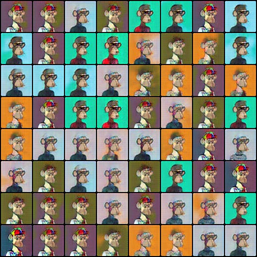
We can see the network progress and a few images are convincing but we are still far from our initial goal

We struggle to avoid model collapse, which is a state in which every generator input leads to the same result.
Some of our limitations are due to our network, which is quite simple and small to current standards.
Link to Code: bit.ly/3T3EHgz
More generated examples: bit.ly/3dIZuGg
If you liked this article I would be super excited if you hit the like button or share it with your curious friends. Anyway, thanks for reading have a great day.